Open an interactive version of this example on Binder:

Forward Reachability

This example demonstrates the forward reachability classifier on a set of dummy data. Note that the data is not taken from a dynamical system, but can easily be adapted to data taken from system observations via a simple substitution. The reason for the dummy data is to showcase the technique on a non-convex forward reachable set.

To run the example, use the following command:

python examples/reach/forward_reach.py

import numpy as np
from functools import partial

import matplotlib
import matplotlib.pyplot as plt

from gym_socks.algorithms.reach.separating_kernel import SeparatingKernelClassifier

from gym_socks.kernel.metrics import abel_kernel
from gym_socks.sampling import sample_fn
from gym_socks.utils.grid import cartesian

/home/docs/checkouts/readthedocs.org/user_builds/socks/envs/develop/lib/python3.9/site-packages/tqdm/auto.py:22: TqdmWarning: IProgress not found. Please update jupyter and ipywidgets. See https://ipywidgets.readthedocs.io/en/stable/user_install.html
  from .autonotebook import tqdm as notebook_tqdm

Generate The Sample

We demonstrate the use of the algorithm on a non-convex region. We choose to sample uniformly within a toroidal region centered around the origin.

@sample_fn
def sampler() -> tuple:
    """Sample generator.

    Sample generator that generates points in a donut-shaped ring around the origin.
    An example of a non-convex region.

    Yields:
        sample : A sample taken iid from the region.

    """

    r = np.random.uniform(low=0.5, high=0.75, size=(1,))
    phi = np.random.uniform(low=0, high=2 * np.pi, size=(1,))
    point = np.array([r * np.cos(phi), r * np.sin(phi)])

    yield tuple(np.ravel(point))


# Sample the distribution.
S = sampler().sample(size=1000)
S = np.array(S)

Algorithm

We then run the algorithm to compute the classification boundary. This can be evaluated easily for a large number of test points.

# Construct the algorithm.
alg = SeparatingKernelClassifier(kernel_fn=partial(abel_kernel, sigma=0.1))

# Generate evaluation (test) points.
x1 = np.linspace(-1, 1, 50)
x2 = np.linspace(-1, 1, 50)
T = cartesian(x1, x2)

# Train the classifier and classify the points.
labels = alg.fit(S).predict(T)

Results

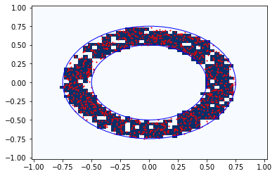
We plot the results here using “pixels” to represent the points predicted to be within the classification boundary. Since the classifier is point-based, it is difficult to plot the “set” defined by the algorithm. Since the set is non-convex, we cannot use a countour plot that relies upon a convex hull.

# Reshape data.
XX, YY = np.meshgrid(x1, x2, indexing="ij")
Z = labels.reshape(XX.shape)

# Plot original data and classified points.
fig = plt.figure()
ax = plt.axes()

plt.pcolor(XX, YY, Z, cmap="Blues", shading="auto")
plt.scatter(S[:, 0], S[:, 1], color="r", marker=".", s=5)

# Plot support region.
plt.gca().add_patch(plt.Circle((0, 0), 0.5, fc="none", ec="blue"))
plt.gca().add_patch(plt.Circle((0, 0), 0.75, fc="none", ec="blue"))

plt.show()

Cite as:

@inproceedings{thorpe2021learning,
  title     = {Learning Approximate Forward Reachable Sets Using Separating Kernels},
  author    = {Thorpe, Adam J. and Ortiz, Kendric R. and Oishi, Meeko M. K.},
  booktitle = {Proceedings of the 3rd Conference on Learning for Dynamics and Control},
  pages     = {201--212},
  year      = {2021},
  volume    = {144},
  series    = {Proceedings of Machine Learning Research},
  month     = {07 -- 08 June},
  publisher = {PMLR},
  pdf       = {http://proceedings.mlr.press/v144/thorpe21a/thorpe21a.pdf},
  url       = {https://proceedings.mlr.press/v144/thorpe21a.html}
}