Open an interactive version of this example on Binder:

A Brief Tutorial on Kernels

Kernel methods are a broad class of statistical learning techniques that leverage functional analysis and reproducing kernel Hilbert spaces (RKHS) to perform classification, clustering, estimation, and regression. Here, we outline the main ideas of kernel methods to help build an intuitive understanding of how kernel methods work.

Basics

What is a kernel?

Intuitively, a kernel is a function that computes the “similarity” between two things. For instance, given two vectors, a kernel tells us how “similar” the two vectors are. This is almost the same as a distance function, which tells us how “close” two things are–but instead of assigning lower values to objects which are close, a kernel typically assigns a higher value to things that are similar.

Mathematically, a kernel is a positive definite function, \(k : \mathcal{X} \times \mathcal{X} \to \mathbb{R}\), meaning given a sample \(\lbrace x_{i} \rbrace_{i=1}^{M}\), the matrix \(G \in \mathbb{R}^{M \times M}\) where \(G_{ij} = k(x_{i}, x_{j})\) is positive semi-definite.

One of the simplest kernels is called the linear kernel, which is defined as the inner product between two things: \(k(x, x') = \langle x, x' \rangle\). But perhaps the most common kernel is the Gaussian kernel, also known as the Radial Basis Function (RBF) kernel,

\[k(x, x') = \exp\biggl(-\frac{\lVert x - x' \rVert^{2}}{2 \sigma^{2}}\biggr)\]

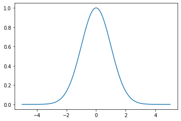
Note that the kernel is a function of two variables. If we fix one of those variables, we effectively center the kernel at a particular value. For instance, with the Gaussian kernel, if we fix one parameter, the Gaussian (mean) becomes centered at that value.

X = np.linspace(-5, 5, 200).reshape(-1, 1)  # Points we want to evaluate at.

x_data = np.array([[0]])  # Gaussian center. Data is organized in rows.
# RBF kernel. Sigma is the "bandwidth" parameter. Larger values give a "wider" kernel.
k = rbf_kernel(X, x_data, sigma=1)

plt.figure()
plt.axes()
plt.plot(X, k)
plt.show()

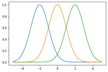
We can add more Gaussians by defining more “centers”.

x_data = np.array([[-2], [0], [2]])

plt.figure()
plt.axes()
plt.plot(X, rbf_kernel(X, x_data, sigma=1))
plt.show()

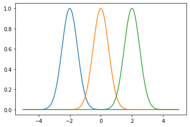
The bandwidth \(\sigma > 0\) of the Gaussian kernel is known as a “hyperparameter”. This is a value we can adjust prior to training, and does not depend explicitly on the data. If we adjust the bandwidth, we get narrower or wider Gaussians.

plt.figure()
plt.axes()
plt.plot(X, rbf_kernel(X, x_data, sigma=0.5))
plt.show()

What are kernel methods?

Kernel methods refers to a broad class of machine learning and statistical learning techniques that are used in a wide variety of applications. At the core, this generally involves learning a function that is represented by kernels.

So imagine we have an unknown function \(f(x) = y\) that we want to learn, but let’s assume that we have some data points \(\lbrace (x_{i}, y_{i}) \rbrace_{i=1}^{M}\) that we’ve observed or that are given to us.

The question we want to ask is: how can we “learn” this function using the data? What we mean is, we want to find some way to represent the function, and we want to incorporate some tunable parameters or values that we can compute. If we tune the parameters appropriately, the representation we have should closely approximate the true function.

For example, we could represent the function by a polynomial, and we use the polynomial coefficients as our tunable parameters. If we represent the function by a line or set of lines, we want to adjust the slope and \(y\)-intersect of those lines to get a good approximation.

This is effectively how all learning works. For instance, neural networks represent a function using a complex system of weights and activation functions.

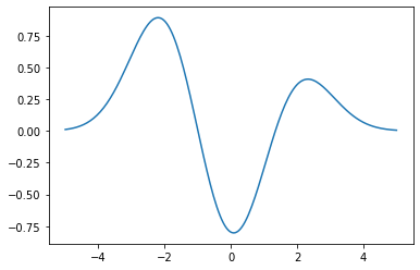
In our case, we represent the function as a linear combination of kernel functions,

\[f(x) = \sum_{i=1}^{M} \alpha_{i} k(x_{i}, x)\]

where \(x_{i}\) are given by our data, and the \(\alpha_{i}\) values are our tunable parameters. In effect, we place a Gaussian kernel at each of our data points \(x_{i}\), and we want to tune the \(\alpha_{i}\) coefficients so that the resulting kernel approximation gives us values that are close to the \(y_{i}\) data points we are given.

Let’s pretend we have some coefficients alpha. Then the kernel approximation is given by,

alpha = np.array([[1], [-1], [0.5]])

plt.figure()
plt.axes()
plt.plot(X, np.dot(rbf_kernel(X, x_data, sigma=1), alpha))
plt.show()

A Practical Example

It’s easy to see that if we are given enough data, and we appropriately choose the coefficients \(\alpha\), then we can closely approximate a function using kernels.

As a practical example, let’s see how this works for a real function,

\[f(x) = x^{3} - 4 x^{2} + 6 x - 24 + \exp(-x)\]

where we assume that we are given data \(\lbrace (x_{i}, y_{i}) \rbrace_{i=1}^{M}\) taken from the function \(f\).

f = lambda x: x ** 3 - 4 * x ** 2 + 6 * x - 24 + np.exp(-x)

X = np.linspace(-5, 5, 200).reshape(-1, 1)  # Points we want to evaluate at.
Y = f(X)  # The actual function values. Used for plotting.

# Our observed data.
sample_size = 5
x_data = np.linspace(-4, 4, sample_size).reshape(-1, 1)
y_data = f(x_data)

For now, we will tune the parameters manually to approximate the function \(f\). We will see shortly, however, that we can compute the coefficients \(\alpha\) directly, without having to manually adjust them.

alpha = np.array([[-110], [-30], [-20], [-20], [0]])

plt.figure()
plt.axis()
plt.plot(X, Y, ":k", label="Actual Function")
plt.plot(X, np.dot(rbf_kernel(X, x_data, sigma=1), alpha), label="Kernel Approximation")
plt.legend()
plt.show()

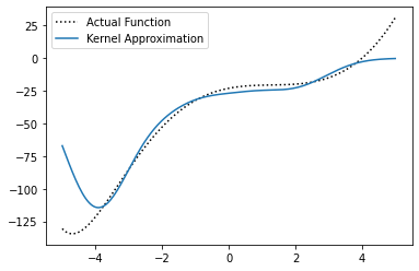
We can see that our approximation is fairly close to the true function, but doesn’t approximate it exactly. If we keep adjusting the parameters \(\alpha\), we could get an even closer approximation. But tuning the coefficients \(\alpha\) by hand can become tedious, especially (as you can imagine) when we have a large amount of data.

Kernel Learning

All learning techniques employ some sort of algorithm to “learn” the tunable parameters in the function representation. For instance, in neural networks we learn the parameters iteratively, by moving them a little bit at a time using a procedure called gradient descent. In order to figure out what direction we need to move the parameters, we define the approximation “error”. Then, the gradient of the error tells us which direction to move the parameters. If we take enough small steps, we will (hopefully) converge to the closest possible approximation, or in other words, the solution with the smallest error.

This is what we mean by “learning”. However, not all learning methods require us to take many small steps to find the “best” values for the parameters or coefficients.

In kernel methods, we don’t need to slowly adjust the parameters over time, and we can directly compute the coefficients that give us the best approximation of our function.

This is because in kernel methods, the error is given by a regularized least squares problem, which has a closed-form solution.

G = rbf_kernel(x_data, sigma=1)
alpha = np.dot(regularized_inverse(G, regularization_param=1e-5, copy=True), y_data)
alpha

array([[-116.69894231],
       [ -34.66770011],
       [ -15.82715869],
       [ -18.04382286],
       [   2.46546819]])

plt.figure()
plt.axis()
plt.plot(X, Y, ":k", label="Actual Function")
plt.plot(X, np.dot(rbf_kernel(X, x_data, sigma=1), alpha), label="Kernel Approximation")
plt.legend()
plt.show()

We can see that the solution is closer to the true function we came up with when we tuned the coefficient manually, and doesn’t require us to manually tune the coefficients \(\alpha\). While it may be slightly better or worse in some specific regions, it is a better approximation overall.

Note that the regularization_param is another hyperparameter (denoted by \(\lambda > 0\)) that is introduced by the regularized least-squares problem, and introduces a little extra error in the solution to keep the function smooth. Ideally, we want this value to be as small as possible. Intuitively, with a small amount of data, the solution can “overfit” to the data points, and won’t be close to the true function in-between the data points we have. Thus, we use \(\lambda\) to prevent overfitting when the dataset is small. However, as the amount of data increases, we can reduce \(\lambda\) to be almost zero, and the extra error becomes negligible.

Here’s the same example with a larger amount of random data.

sample_size = 100
x_data = 8 * np.random.rand(sample_size, 1) - 4  # Random data in (-4, 4)
y_data = f(x_data)

G = rbf_kernel(x_data, sigma=1)
alpha = np.dot(regularized_inverse(G, regularization_param=1e-9), y_data)

plt.figure()
plt.axis()
plt.scatter(x_data, y_data, s=5, c="red", label="Data")
plt.plot(X, Y, ":k", label="Actual Function")
plt.plot(X, np.dot(rbf_kernel(X, x_data, sigma=1), alpha), label="Kernel Approximation")
plt.legend()
plt.show()

We can see that as the amount of data increases, our approximation gets very close to the true function.

What is an RKHS?

A reproducing kernel Hilbert space (RKHS) is effectively a function space defined by the kernel. When we choose a kernel function, we are specifying what the functions in the RKHS look like. For instance, when we choose a Gaussian kernel, the associated RKHS is the set of all functions that can be represented by a linear combination of Gaussians. If we use a polynomial kernel, then the associated RKHS is the set of all polynomials of a certain order.

When we dive into the math of reproducing kernel Hilbert spaces, things can become daunting very quickly since it involves a significant amount of functional analysis. This deters many people from using kernel methods or studying them, since the math is considered too “hard”. However, this should not be the case, as the concept of an RKHS is superficially very easy to grasp.

Advanced Topics

Here, we’ve given a basic understanding of kernel methods and how kernels can be used for function approximation. However, we’ve barely scratched the surface when it comes to the ways in which kernels can be used. For those who are interested in learning more about the techniques used in SOCKS, or simply want to learn more about kernel methods, we’ve provided some tutorials on some advanced topics. These tutorials are geared toward those who already have a background in machine learning, but may not be as familiar with kernel methods.

• RKHS Tutorial
• Statistical Learning
• Neural Network vs. Kernels

Also, be sure to check out the examples page for a showcase of the algorithms in SOCKS.