Open an interactive version of this example on Binder:

Statistical Learning

In this tutorial, we will briefly cover some of the techniques that we employ in SOCKS. In a previous tutorial, we covered the basics of kernels and described how kernel methods can be used for function approximation.

To recap, here is the example from the previous tutorial.

f = lambda x: x ** 3 - 4 * x ** 2 + 6 * x - 24 + np.exp(-x)

X = np.linspace(-5, 5, 200).reshape(-1, 1)  # Points we want to evaluate at.
Y = f(X)  # The actual function values. Used for plotting.

sample_size = 100
x_data = 8 * np.random.rand(sample_size, 1) - 4  # Random data in (-4, 4)
y_data = f(x_data)

G = rbf_kernel(x_data, sigma=1)
alpha = np.dot(regularized_inverse(G, regularization_param=1e-9), y_data)

plt.figure()
plt.axis()
plt.scatter(x_data, y_data, s=5, c="red", label="Data")
plt.plot(X, Y, ":k", label="Actual Function")
plt.plot(X, np.dot(rbf_kernel(X, x_data, sigma=1), alpha), label="Kernel Approximation")
plt.legend()
plt.show()

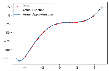
Here, we collect data from a function, with points taken randomly in \(x\), and we compute the kernel-based approximation as the solution to a regularized least-squares problem. However, note that the data we collect \(\lbrace (x_{i}, y_{i}) \rbrace_{i=1}^{M}\) is not corrupted by any noise.

Noisy Measurements

What happens when we add some noise to the outputs of our function data?

sample_size = 100
x_data = 8 * np.random.rand(sample_size, 1) - 4  # Random data in (-4, 4)
# Add Gaussian noise to the data.
y_data = f(x_data) + 10 * np.random.randn(sample_size, 1)

# Points to evaluate our kernel approximation at.
x_eval = np.linspace(-5, 5, 200).reshape(-1, 1)

# Compute the kernel-based approximation.
G = rbf_kernel(x_data, sigma=1)
y_pred = (
    y_data.T
    @ regularized_inverse(G, regularization_param=1e-3)
    @ rbf_kernel(x_data, x_eval, sigma=1)
)

plt.figure()
plt.axis()
plt.scatter(x_data, y_data, s=5, c="red", label="Data")
plt.plot(X, Y, ":k", label="Actual Function")
plt.plot(x_eval, y_pred.T, label="Kernel Approximation")
plt.legend()
plt.show()

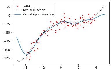
We can see that the function that we learn still fits the noisy data (though not as well), but we need to raise the regularization parameter to keep the solution “smooth”. Clearly, the quality of the approximation depends on the data. If we have too much noise in a particular region, or not enough data, the approximation will be poor. We can improve the quality of the approximation by increasing the sample size.

sample_size = 500
x_data = 8 * np.random.rand(sample_size, 1) - 4  # Random data in (-4, 4)
# Add Gaussian noise to the data.
y_data = f(x_data) + 10 * np.random.randn(sample_size, 1)

# Points to evaluate our kernel approximation at.
x_eval = np.linspace(-5, 5, 200).reshape(-1, 1)

# Compute the kernel-based approximation.
G = rbf_kernel(x_data, sigma=1)
y_pred = (
    y_data.T
    @ regularized_inverse(G, regularization_param=1e-3)
    @ rbf_kernel(x_data, x_eval, sigma=1)
)

plt.figure()
plt.axis()
plt.scatter(x_data, y_data, s=5, c="red", label="Data")
plt.plot(X, Y, ":k", label="Actual Function")
plt.plot(x_eval, y_pred.T, label="Kernel Approximation")
plt.legend()
plt.show()

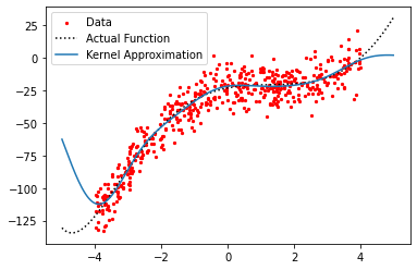
Now, it is important to ask, what exactly are we learning here?

Since the function outputs are corrupted by noise, we are working with a stochastic function, meaning it incorporates some randomness. The answer, then, is that we are learning the expectation of the stochastic function.

In short, if we were to evaluate the stochastic function at the same value of \(x\) over and over, we would get different random values for \(y\). Thus, if we were simply trying to find the “best fit” function to the random data, we would not actually be fitting the underlying function.

Instead, we are attempting to learn an approximation of the function that gives us the most likely value of \(y\) for every value of \(x\). In probability theory, this is called the expected value or expectation.

Probability Distributions

When we are dealing with random variables and stochasticity, we have what is called a distribution, which maps probabilities to outcomes. The distribution also tells us which outcome is the most likely, and this is effectively the expectation.

Mathematically, we write this as,

\[\mathbb{E}[f(X)]\]

Now, if \(f\) is a function in an RKHS, we can actually write this using the reproducing property (see here) as the inner product between the function \(f\) and another element in the RKHS which we call the kernel distribution embedding.

\[\mathbb{E}[f(X)] = \langle f, m(X) \rangle\]

We can compute the expectation at \(X = x\) if we fix the random variable \(X\) to a particular value \(x\).

This means that what we are trying to learn is the embedding \(m\) in the RKHS.

Note

This is a very simple explanation of distributions and expectations, and we have avoided a more involved explanation to avoid confusion. Mathematically, these concepts have much more involved definitions. For those who work with stochasticity or probability in continuous spaces, we highly recommend checking out a book on measure theory.

Learning Embeddings

Since the embedding \(m\) is an element of the RKHS, it can be represented as a linear combination of kernel functions, just as we did before.

In practice, this means that the same techniques we used to compute the kernel-based approximation still apply. However, we need to think a little more deeply about what we are actually trying to learn when stochasticity and distributions are involved.

References

Kernel embeddings of distributions is a deep topic. Here, we provide a list of some relevant references to get started with kernel embeddings.

• Alex Smola, Arthur Gretton, Le Song, and Bernhard Schölkopf. A Hilbert space embedding for distributions. In Proceedings of the 18th International Conference on Algorithmic Learning Theory, ALT '07, 13–31. Berlin, Heidelberg, 2007. Springer-Verlag. doi:10.1007/978-3-540-75225-7_5.

• Le Song, Jonathan Huang, Alex Smola, and Kenji Fukumizu. Hilbert space embeddings of conditional distributions with applications to dynamical systems. In Proceedings of the 26th Annual International Conference on Machine Learning, ICML '09, 961–968. New York, NY, USA, 2009. Association for Computing Machinery. doi:10.1145/1553374.1553497.

• Krikamol Muandet, Kenji Fukumizu, Bharath Sriperumbudur, and Bernhard Schölkopf. Kernel mean embedding of distributions: a review and beyond. Foundations and Trends® in Machine Learning, 10(1-2):1–141, 2017. doi:10.1561/2200000060.

• Steffen Grünewälder, Guy Lever, Luca Baldassarre, Massimilano Pontil, and Arthur Gretton. Modelling transition dynamics in mdps with rkhs embeddings. In Proceedings of the 29th International Coference on Machine Learning, ICML'12, 1603–1610. Madison, WI, USA, 2012. Omnipress.

• Le Song, Kenji Fukumizu, and Arthur Gretton. Kernel embeddings of conditional distributions: a unified kernel framework for nonparametric inference in graphical models. IEEE Signal Processing Magazine, 30(4):98–111, 2013. doi:10.1109/MSP.2013.2252713.

• Steffen Grünewälder, Guy Lever, Luca Baldassarre, Sam Patterson, Arthur Gretton, and Massimilano Pontil. Conditional mean embeddings as regressors. In Proceedings of the 29th International Conference on Machine Learning, ICML'12, 1803–1810. Madison, WI, USA, 2012. Omnipress.