Open an interactive version of this example on Binder:

Nystrom Approximation

This example demonstrates the use of conditional distribution embeddings on a simple function \(x^{2}\), corrupted by Gaussian noise and using the Nystrom kernel approximation technique. This example is useful for experimenting with the kernel choice, parameters, or dataset and visualizing the result.

The Nystrom method computes an approximation of the Gram matrix that uses a subset of the data. By identifying the primary components of the data, we can obtain a more efficient approximation of the Gram matrix. This is useful when working with the Gram matrix directly, but may not offer significant savings for conditional embeddings, since the matrix inverse operation is the primary source of computational complexity, and the Nystrom approximation has the same size as the original Gram matrix.

To run the example, use the following command:

python examples/kernel/nystrom_approximation.py

import numpy as np
from functools import partial
from gym_socks.algorithms.kernel import ConditionalEmbedding

from gym_socks.kernel.metrics import rbf_kernel
from gym_socks.kernel.metrics import woodbury_inverse

from sklearn.kernel_approximation import Nystroem

from time import perf_counter

Generate the Sample

sample_size = 200
X_train = np.random.uniform(-5.5, 5.5, sample_size).reshape(-1, 1)
y_train = X_train ** 2
y_train += 2 * np.random.standard_normal(size=(sample_size, 1))  # Additive noise.

X_test = np.linspace(-5, 5, 1000).reshape(-1, 1)

Kernel and Parameters

• The regularization parameter affects the “smoothness” of the approximation. If the value is too low, this will lead to overfitting. If the value is high, the approximation may be overly smooth.

• For the Gaussian (RBF) kernel, sigma controls the “bandwidth” of the Gaussian. Decreasing this will allow the approximation to detect sharper changes in the function, while a larger value will give a smoother approximation.

• num_features controls the number of samples used to approximate the kernel matrix.

sigma = 1
gamma = 1 / (2 * (sigma ** 2))
kernel_fn = partial(rbf_kernel, sigma=sigma)
regularization_param = 1 / (sample_size ** 2)
num_features = 100  # Number of features.

Compute the Nystrom Approximation

Note that the time savings is seen primarily when we need to work with and manipulate the Gram matrix, since we obtain a feature map \(\Phi\) such that \(\hat{G} = \Phi \Phi^{\top}\). However, this does not help much with the matrix inverse operations since the approximated Gram matrix has the same dimensionality as the original.

start = perf_counter()
alg = ConditionalEmbedding(regularization_param=regularization_param)
nystroem_sampler = Nystroem(
    kernel="rbf", gamma=gamma, n_components=num_features, random_state=1
)

Z_train = nystroem_sampler.fit_transform(X_train)

y_pred = alg.fit(Z_train @ Z_train.T, y_train).predict(kernel_fn(X_train, X_test))
print(perf_counter() - start)

0.01828857300006348

Plot the Results

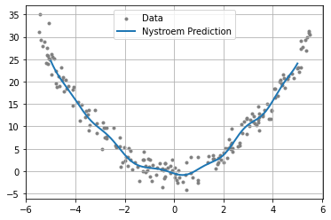
We then plot the results using the approximation of the Gram matrix computed using the Nystrom method.

import matplotlib
from matplotlib import pyplot as plt

fig = plt.figure()
ax = plt.axes()
plt.grid()

plt.scatter(X_train, y_train, marker=".", c="grey", label="Data")
plt.plot(X_test, y_pred, linewidth=2, label="Nystroem Prediction")

plt.legend()

plt.show()

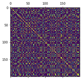
Comparing the Gram matrix approximation with the actual Gram matrix.

plt.matshow(kernel_fn(X_train))
plt.matshow(Z_train @ Z_train.T)

plt.show()

Using the Woodbury Matrix Identity

Because we have an explicit feature map \(\Phi\), and the matrix inverse term is computed via \((\Phi \Phi^{\top} + \lambda M I)^{-1}\), we can use the Woodbury matrix identity to perform a faster computation of the conditional distribution embedding.

\[(A + U C V)^{-1} = A^{-1} - A^{-1} U (C^{-1} + V A^{-1} U)^{-1} V A^{-1}\]

The following result should be faster than the method above, since we have a smaller matrix inversion that scales with the number of features.

start = perf_counter()
alg = ConditionalEmbedding(regularization_param=regularization_param)
nystroem_sampler = Nystroem(
    kernel="rbf", gamma=gamma, n_components=num_features, random_state=1
)

Z_train = nystroem_sampler.fit_transform(X_train)

A = np.zeros((sample_size, sample_size))
np.fill_diagonal(A, 1 / (regularization_param * sample_size))

C = np.identity(num_features)

# D = np.linalg.inv(C + (Z_train.T @ A @ Z_train))
# W = A - (A @ Z_train @ D @ Z_train.T @ A)
W = woodbury_inverse(A, Z_train, C, Z_train.T, precomputed=True)

y_pred_woodbury = (y_train.T @ W @ kernel_fn(X_train, X_test)).T

print(perf_counter() - start)

0.01377354399937758

Plot the Result

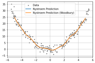
We then plot the approximation computed using the Woodbury matrix identity against the original result to verify that they are equal.

fig = plt.figure()
ax = plt.axes()
plt.grid()

plt.scatter(X_train, y_train, marker=".", c="grey", label="Data")
plt.plot(X_test, y_pred, linewidth=2, label="Nystroem Prediction")
plt.plot(X_test, y_pred_woodbury, linewidth=2, label="Nystroem Prediction (Woodbury)")

plt.legend()

plt.show()