Open an interactive version of this example on Binder:

Conditional Distribution Embedding

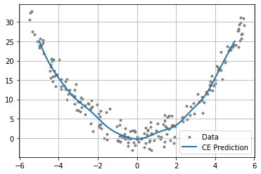
This example demonstrates the use of conditional distribution embeddings on a simple function \(x^{2}\), corrupted by Gaussian noise. This example is useful for experimenting with the kernel choice, parameters, or dataset and visualizing the result.

To run the example, use the following command:

python examples/kernel/conditional_embedding.py

import numpy as np
from functools import partial
from gym_socks.algorithms.kernel import ConditionalEmbedding
from gym_socks.kernel.metrics import rbf_kernel

from time import perf_counter

Generate the Sample

sample_size = 200
X_train = np.random.uniform(-5.5, 5.5, sample_size).reshape(-1, 1)
y_train = X_train ** 2
y_train += 2 * np.random.standard_normal(size=(sample_size, 1))  # Additive noise.

X_test = np.linspace(-5, 5, 1000).reshape(-1, 1)

Kernel and Parameters

• The regularization parameter affects the “smoothness” of the approximation. If the value is too low, this will lead to overfitting. If the value is high, the approximation may be overly smooth.

• For the Gaussian (RBF) kernel, sigma controls the “bandwidth” of the Gaussian. Decreasing this will allow the approximation to detect sharper changes in the function, while a larger value will give a smoother approximation.

sigma = 1
kernel_fn = partial(rbf_kernel, sigma=sigma)
regularization_param = 1 / (sample_size ** 2)

Compute the Appromation

We now compute the estimated \(y\) values of the function at new (unseen) values of \(x\).

start = perf_counter()
alg = ConditionalEmbedding(regularization_param=regularization_param)

y_pred = alg.fit(kernel_fn(X_train), y_train).predict(kernel_fn(X_train, X_test))
print(perf_counter() - start)

0.010211563000666501

Plot the Results

We then plot the results and the original data.

import matplotlib
from matplotlib import pyplot as plt

fig = plt.figure()
ax = plt.axes()
plt.grid()

plt.scatter(X_train, y_train, marker=".", c="grey", label="Data")
plt.plot(X_test, y_pred, linewidth=2, label="CE Prediction")

plt.legend()

plt.show()