Open an interactive version of this example on Binder:

Target Tracking (Translation and Rotation Invariance)

This example demonstrates the kernel-based stochastic optimal control algorithm on a nonholonomic vehicle system (unicycle dynamics), and seeks to track a v-shaped trajectory. In this example, we exploit the properties of the dynamical system to more efficiently sample from the state space.

To run the example, use the following command:

python examples/control/tracking.py

The main problem is that the kernel function measures similarity based on the entire state vector. Given two systems that are separated by some distance, but otherwise identical, we might expect the sample information from one system to be useful in determining the dynamics of the other. For instance, if we collect sample information from a car, the sample information might be relevant even if we started several feet to the left or right. However, because the kernel naively measures similarity based on all state variables, it generally does not capture the translation (or rotation) invariance properties of the dynamical system.

In other words, unless we collect sample information globally, we can easily enter a region for which no data is available.

One possible approach is to exploit the known properties of the system dynamics, specifically the translation invariance and rotation invariance properties, which tell us that the dynamics corresponding to particular state variables do not change if the state is shifted or rotated. In a deterministic setting (no randomness), if we apply a control action to a system from some initial condition, and observe the resulting state, then translation invariance means that applying the same control action to a shifted initial condition would lead to a resulting state that is shifted by the same amount.

By exploiting these properties, we can collect a sample from a smaller region of the state space, and then using translations and rotations, we can “move” the sample to the region we are currently operating in. In effect, this serves to reduce the overall amount of sample information needed to characterize the dynamics.

import gym

import numpy as np

from gym_socks.envs.nonholonomic import NonholonomicVehicleEnv

from functools import partial
from itertools import islice

from gym_socks.kernel.metrics import rbf_kernel

from gym_socks.sampling import sample_fn
from gym_socks.sampling import space_sampler
from gym_socks.sampling.transform import transpose_sample

import matplotlib
import matplotlib.pyplot as plt

Demonstration of the Idea

In order to demonstrate the idea, we can look at a deterministic system.

class DeterministicNonholonomicVehicleEnv(NonholonomicVehicleEnv):
    def generate_disturbance(self, time, state, action):
        return np.zeros(shape=self.state_space.shape)


deterministic_env = DeterministicNonholonomicVehicleEnv()

# Generate a collection of random actions.
action_sample_space = gym.spaces.Box(
    low=np.array([0.1, -10.1], dtype=np.float32),
    high=np.array([1.1, 10.1], dtype=np.float32),
    shape=deterministic_env.action_space.shape,
    dtype=deterministic_env.action_space.dtype,
)
random_actions = space_sampler(action_sample_space).sample(size=100)

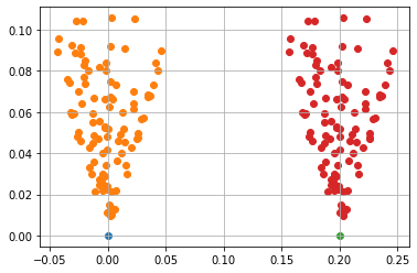
Translation Invariance

Consider the nonholonomic vehicle system above. If we look at a car model and apply an action to the vehicle, it generally does not matter if the car started slightly to the left or right. The action would have produced a similar result, regardless of the \(x\) or \(y\) position of the vehicle.

# Simulate the system from one initial condition.

resulting_states1 = []
initial_condition1 = [0, 0, 0]
for action in random_actions:
    deterministic_env.reset(initial_condition1)
    deterministic_env.step(action=action)
    resulting_states1.append(deterministic_env.state)

resulting_states2 = []
initial_condition2 = [0.2, 0, 0]
for action in random_actions:
    deterministic_env.reset(initial_condition2)
    deterministic_env.step(action=action)
    resulting_states2.append(deterministic_env.state)

fig = plt.figure()
ax = plt.axes()
plt.grid()

resulting_states1 = np.array(resulting_states1)
plt.scatter(initial_condition1[0], initial_condition1[1])
plt.scatter(resulting_states1[:, 0], resulting_states1[:, 1])

resulting_states2 = np.array(resulting_states2)
plt.scatter(initial_condition2[0], initial_condition2[1])
plt.scatter(resulting_states2[:, 0], resulting_states2[:, 1])

plt.show()

Rotation Invariance

In addition, it generally does not matter what direction the vehicle is pointing. No matter the steering angle (heading) of the vehicle, the dynamics operate in a similar fashion.

resulting_states1 = []
initial_condition1 = [0, 0, 0]
for action in random_actions:
    deterministic_env.reset(initial_condition1)
    deterministic_env.step(action=action)
    resulting_states1.append(deterministic_env.state)

resulting_states2 = []
initial_condition2 = [0, 0, np.pi / 2]
for action in random_actions:
    deterministic_env.reset(initial_condition2)
    deterministic_env.step(action=action)
    resulting_states2.append(deterministic_env.state)

fig = plt.figure()
ax = plt.axes()
plt.grid()

resulting_states1 = np.array(resulting_states1)
plt.scatter(initial_condition1[0], initial_condition1[1])
plt.scatter(resulting_states1[:, 0], resulting_states1[:, 1])

resulting_states2 = np.array(resulting_states2)
plt.scatter(initial_condition2[0], initial_condition2[1])
plt.scatter(resulting_states2[:, 0], resulting_states2[:, 1])

plt.show()

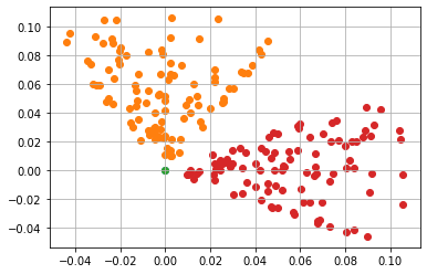
Thus, we can use a random sample that is translated and rotated in order to approximate the dynamics more globally.

Generate the Sample

sigma = 1.5  # Kernel bandwidth parameter.
regularization_param = 1e-5  # Regularization parameter.
kernel_fn = partial(rbf_kernel, sigma=sigma)

time_horizon = 20

# For controlling randomness.
seed = 12345

We generate a random sample from the system, and choose random control actions from a single initial condition (the origin). Alternatively, we could translate the sample information while we generate it from random initial conditions.

NOTE: We use significantly less sample information to obtain a similar result to the tracking example. Here, since we can translate and rotate the sample, we use 100 sample points, wehre in the other example we use 1,500 by default to obtain similar behavior.

env = NonholonomicVehicleEnv()
env.seed(seed)

sample_size = 100

action_sample_space = gym.spaces.Box(
    low=np.array([0.1, -10.1], dtype=np.float32),
    high=np.array([1.1, 10.1], dtype=np.float32),
    shape=env.action_space.shape,
    dtype=env.action_space.dtype,
    seed=seed,
)
action_sampler = space_sampler(action_sample_space)


@sample_fn
def custom_sampler():
    state = np.array([0.0, 0.0, 0.0])
    action = next(action_sampler)

    env.reset(state)
    env.step(action=action)
    next_state = env.state

    yield state, action, next_state


S = custom_sampler().sample(size=sample_size)
A = action_sampler.sample(size=sample_size)

X, U, Y = transpose_sample(S)

X = np.array(X)
U = np.array(U)
Y = np.array(Y)

Compute the Kernel Matrices

We then compute the kernel matrices needed to compute the optimal control actions.

One advantage of the translation and rotation invariant approach is that since the initial conditions are set to zero, which we can do since the nonholonomic vehicle is translation and rotation invariant, the Gram matrix for the X vectors is a matrix of all ones using the RBF kernel. Thus, we can omit it from our calculations, which greatly simplifies the implementation of the control algorithm.

G = kernel_fn(U)
b = np.linalg.solve(
    (G + sample_size * regularization_param * np.identity(sample_size)), kernel_fn(U, A)
)

Generate the Target Trajectory

We define the cost as the norm distance to the target at each time step.

a = 0.5  # Path amplitude.
p = 2.0  # Path period.
target_trajectory = [
    [
        (x * 0.1) - 1.0,
        4 * a / p * np.abs((((((x * 0.1) - 1.0) - p / 2) % p) + p) % p - p / 2) - a,
    ]
    for x in range(time_horizon)
]


def _tracking_cost(time: int = 0, state: np.ndarray = None) -> float:
    """Tracking cost function.

    The goal is to minimize the distance of the x/y position of the vehicle to the
    'state' of the target trajectory at each time step.

    Args:
        time : Time of the simulation. Used for time-dependent cost functions.
        state : State of the system.

    Returns:
        cost : Real-valued cost.

    """

    state = np.atleast_1d(state)

    YT = Y

    # Rotation invariant shift.
    theta = state[2]
    YT[:, 2] += theta
    # Rotation matrix.
    R = np.array(
        [
            [np.cos(theta), -np.sin(theta), 0],
            [np.sin(theta), np.cos(theta), 0],
            [0, 0, 1],
        ],
        dtype=np.float32,
    )
    YT = YT @ R

    # Translation invariant shift.
    YT[:, :2] += state[:2]

    dist = YT[:, :2] - np.array([target_trajectory[time]])
    result = np.linalg.norm(dist, ord=2, axis=1)
    result = np.power(result, 2)
    return result

Simulate the Controlled System

We then simulate the system forward in time, choosing the appropriate control actions at each time step.

env.reset()
initial_condition = [-0.8, 0, 0]
env.reset(initial_condition)
trajectory = [initial_condition]

for t in range(time_horizon):
    # Compute the control action.
    C = _tracking_cost(time=t, state=env.state) @ b
    idx = np.argmin(C)
    action = A[idx]

    state, *_ = env.step(time=t, action=action)

    trajectory.append(list(state))

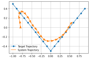
Results

We then plot the simulated trajectory of the system alongside the target trajectory.

fig = plt.figure()
ax = plt.axes()
plt.grid()

target_trajectory = np.array(target_trajectory, dtype=np.float32)
plt.plot(
    target_trajectory[:, 0],
    target_trajectory[:, 1],
    marker="o",
    color="C0",
    label="Target Trajectory",
)

trajectory = np.array(trajectory, dtype=np.float32)
plt.plot(
    trajectory[:, 0],
    trajectory[:, 1],
    color="C1",
    label="System Trajectory",
)

# Plot the markers as arrows, showing vehicle heading.
paper_airplane = [(0, -0.25), (0.5, -0.5), (0, 1), (-0.5, -0.5), (0, -0.25)]

for x in trajectory:
    angle = -np.rad2deg(x[2])

    t = matplotlib.markers.MarkerStyle(marker=paper_airplane)
    t._transform = t.get_transform().rotate_deg(angle)

    plt.plot(x[0], x[1], marker=t, markersize=15, linestyle="None", color="C1")

plt.legend()
plt.show()