Open an interactive version of this example on Binder:

Generative Model

This example demonstrates the use of kernel embeddings to construct a generative model.

When we compute the kernel distribution embedding, it should be noted that the embedding is the best fit function in the RKHS for the given data (and given the hyperparameters \(\sigma\) and \(\lambda\)). As the amount of data increases and the regularization parameter \(\lambda\) tends to \(0\), we obtain a closer approximation of the true embedding. However, for a finite sample, this is simply an approximation of the true embedding. If we were given different data drawn from the same distribution, then the (empirical) embedding would change.

Nevertheless, we expect that with different training data, the approximation we obtain should be close to the empirical embedding in the RKHS using the actual, observed data points we have. Mathematically, this can be described as being close to the empirical embedding in the RKHS norm.

We define a ball in the Hilbert space \(\lbrace f \in \mathscr{H} \mid \lVert f - m \rVert_{\mathscr{H}} \leq r \rbrace\), where \(m\) is the empirical embedding that matches the data and \(r\) is the radius of the ball. The generative model we construct can be viewed as randomly generating functions in the RKHS that are close to the empirical embedding in the RKHS norm. In other words, we generate functions,

\[g \sim U(\lbrace f \in \mathscr{H} \mid \lVert f - m \rVert_{\mathscr{H}} \leq r \rbrace)\]

where \(U\) denotes a uniform distribution over the RKHS ball.

To run the example, use the following command:

python examples/experimental/generative_model.py

Graphical Explanation

This figure shows the norm ball in the RKHS.

The red dot indicates the true embedding and the maximum error (distance) in probability \(\epsilon\) (red line) to the empirical embedding (blue dot). The larger ball is the RKHS ball where the generator samples from. The blue line depicts the diameter of the RKHS ball. This indicates that if we seek to generate functions which are still close to the true embedding, that the ball should be chosen to have radius \(2 \epsilon\) (which would have a maximum error in probability of \(3 \epsilon\) from the true embedding).

Demonstration of the Idea

import numpy as np
from functools import partial

from gym_socks.algorithms.kernel import GenerativeModel
from gym_socks.kernel.metrics import rbf_kernel

from time import perf_counter

import matplotlib
from matplotlib import pyplot as plt

Generate the Sample

We generate a finite sample taken from a simple function \(x^{2}\), corrupted by Gaussian noise to compute the embedding and for plotting purposes.

sample_size = 200
X_train = np.random.uniform(-5.5, 5.5, sample_size).reshape(-1, 1)
y_train = X_train ** 2
y_train += 2 * np.random.standard_normal(size=(sample_size, 1))  # Additive noise.

X_test = np.linspace(-5, 5, 1000).reshape(-1, 1)

Kernel and Parameters

We then define the kernel and the regularization parameter. The value \(\sigma\) is the “bandwidth” parameter of the Gaussian (RBF) kernel and \(\lambda\) is the regularization parameter. Increasing these values should lead to a smoother approximation.

sigma = 1
kernel_fn = partial(rbf_kernel, sigma=sigma)
regularization_param = 1 / (sample_size ** 2)

Compute the Appromation

We now compute the estimated \(y\) values of the function at new (unseen) values of \(x\), as well as generate a number of functions that are close in the RKHS norm to the empirical embedding.

start = perf_counter()
num_samples = 10  # Number of generated functions.

alg = GenerativeModel(regularization_param=regularization_param)
G = kernel_fn(X_train)
K = kernel_fn(X_train, X_test)

# Fit the gerneative model to the data.
alg.fit(G, y_train)

# Compute the conditional distribution embedding. Used for plotting.
y_mean = alg.predict(K)

# Compute the predicted y values for the generated functions.
y_pred = alg.sample(K, num_samples, radius=4)

print(perf_counter() - start)

0.011311236999972607

Tip

We can decrease the “variability” of the functions we generate by reducing the radius. Here, we choose radius=4 to mimic the noise process.

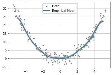
Plot the Results

We then plot the results and the original data.

fig = plt.figure()
ax = plt.axes()
plt.grid()

plt.scatter(X_train, y_train, marker=".", c="grey", label="Data")

# Plot the y values from the generated functions.
plt.plot(X_test, y_pred.T, alpha=0.5, linewidth=1)

# Plot the conditional distribution embedding.
plt.plot(X_test, y_mean, linewidth=2, label="Empirical Mean")

plt.legend()

plt.show()

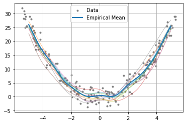
We see that the generative model produces functions which could potentially describe the observed data. This may be useful in a learning context where only sparse data is avilable.

Possible Use Cases

Here, we outline some possible use cases for this model.

• Generating artificial trajectories for a dynamical system that are close to the observed trajectories.

• Generating alternative control sequences for the purpose of synthesizing controllers.

• Testing robustness of control solutions.

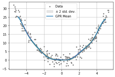
Comparison with GPs

A Gaussian process (GP) can be used as a kind of generative model. In short, given data, we can compute the mean and covariance of the Gaussian process (note that the mean function is virtually identical to the conditional distribution embedding), and using the covariance, we can generate functions from the GP.

However, this approach has one significant drawback. The covariance function can be overly restrictive, particularly in high-noise scenarios like the one we demonstrate here. Because of the relative data density and high noise, the generative model only returns functions which are very close to the mean. Additionally, note that we have to keep the regularization parameter \(\lambda\) high (alpha in the code below) in order to avoid too much noise in our generated functions.

Another way to look at this is: GP models have very low covariance around observed data, meaning the generated functions will be “close” to the observed points, but may vary more substantially in areas where data is unavailable.

However, the observed data may be far away from the true mean, since it itself is corrupted by noise. Thus, the functions which are generated by the GP being close to the observed points may actually be detrimental.

from sklearn.gaussian_process import GaussianProcessRegressor
from sklearn.gaussian_process.kernels import RBF

x = np.linspace(-5, 5, 1000)
X_test = x.reshape(-1, 1)

gpr = GaussianProcessRegressor(RBF(sigma, length_scale_bounds="fixed"), alpha=1)
gpr.fit(X_train, y_train)

y_mean, y_std = gpr.predict(X_test, return_std=True)
y_pred_gpr = gpr.sample_y(X_test, n_samples=num_samples)

fig = plt.figure()
ax = plt.axes()
plt.grid()

plt.scatter(X_train, y_train, marker=".", c="grey", label="Data")

# Plot the standard deviation.
plt.fill_between(
    x,
    np.squeeze(y_mean) - 2 * y_std,
    np.squeeze(y_mean) + 2 * y_std,
    alpha=0.1,
    color="black",
    label=r"$\pm$ 2 std. dev.",
)

# Plot the y values from the generated functions.
plt.plot(X_test, np.squeeze(y_pred_gpr), alpha=0.5, linewidth=1)

# Plot the GPR mean function.
plt.plot(X_test, y_mean, linewidth=2, label="GPR Mean")

plt.legend()

plt.show()

Try It

We demonstrate here a particular case where Gaussian processes may not work well as a generative process. Try changing the parameters alpha, the kernel parameter, as well as the kernel function itself to see the effects.

We can achieve a similar effect to the GP generative process using our proposed approach by reducing the radius of the ball in Hilbert space.

regularization_param = 1e-2

alg = GenerativeModel(regularization_param=regularization_param)
alg.fit(G, y_train)

y_mean = alg.predict(K)  # For plotting.

y_pred = alg.sample(K, num_samples, radius=1)

fig = plt.figure()
ax = plt.axes()
plt.grid()

plt.scatter(X_train, y_train, marker=".", c="grey", label="Data")

# Plot the y values from the generated functions.
plt.plot(X_test, y_pred.T, alpha=0.5, linewidth=1)

plt.plot(X_test, y_mean, linewidth=2, label="Empirical Mean")

plt.legend()
plt.show()