Open an interactive version of this example on Binder:

Stochastic Reachability

This example shows the stochastic reachability algorithm.

By default, the system is a double integrator (2D stochastic chain of integrators).

To run the example, use the following command:

python examples/reach/stoch_reach.py

import gym

import numpy as np

from functools import partial

from gym.envs.registration import make
from sklearn.metrics.pairwise import rbf_kernel

from gym_socks.algorithms.reach.kernel_sr import kernel_sr

from gym_socks.sampling import sample
from gym_socks.sampling import default_sampler
from gym_socks.sampling import grid_sampler
from gym_socks.sampling import repeat

from gym_socks.utils.grid import make_grid_from_space
from gym_socks.utils.grid import make_grid_from_ranges

Configuration variables.

system_id = "2DIntegratorEnv-v0"
time_horizon = 5
sigma = 0.1
regularization_param = 1

Generate The Sample

We demonstrate the algorithm on a simple 2-D integrator system, and sample on a grid within the region of interest. Note that this is a simplification in order to make the result look more “uniform”, but is not specifically required for the algorithm to work.

env = make(system_id)

sample_size = 3125  # This number is chosen based on the values below.

sample_space = gym.spaces.Box(
    low=-1.1, high=1.1, shape=env.state_space.shape, dtype=env.state_space.dtype
)

state_sampler = repeat(
    grid_sampler(make_grid_from_space(sample_space=sample_space, resolution=25)), num=5
)

action_sampler = grid_sampler(make_grid_from_ranges([np.linspace(-1, 1, 5)]))

S = sample(
    sampler=default_sampler(
        state_sampler=state_sampler, action_sampler=action_sampler, env=env
    ),
    sample_size=sample_size,
)

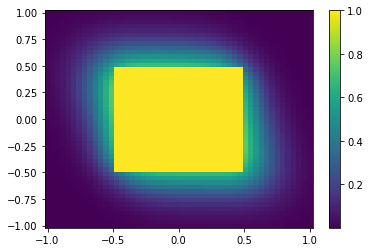
We define the target tube and the constraint (safety) tube, which are sequences of bounded sets indexed by time. Here, we define the target tube such that it is between -0.5 and 0.5, and specify the constraint tube to be between -1 and 1.

target_tube = [
    gym.spaces.Box(low=-0.5, high=0.5, shape=(2,), dtype=np.float32)
] * time_horizon

constraint_tube = [
    gym.spaces.Box(low=-1, high=1, shape=(2,), dtype=np.float32)
] * time_horizon

# Generate test points.
x1 = np.linspace(-1, 1, 50)
x2 = np.linspace(-1, 1, 50)
T = make_grid_from_ranges([x1, x2])

Algorithm

We then run the algorithm to compute the safety probabilities at each of the test points for the first-hitting time stochastic reachability problem. We can easily change to the terminal-hitting time problem by changing “FHT” below to “THT”.

safety_probabilities = kernel_sr(
    S=S,
    T=T,
    time_horizon=time_horizon,
    constraint_tube=constraint_tube,
    target_tube=target_tube,
    problem="FHT",
    regularization_param=regularization_param,
    kernel_fn=partial(rbf_kernel, gamma=1 / (2 * (sigma ** 2))),
    verbose=False,
)

Results

We then plot the results for all of the test points. The warmer colors indicate higher safety probabilities.

import matplotlib
import matplotlib.pyplot as plt

# Reshape data.
XX, YY = np.meshgrid(x1, x2, indexing="ij")
Z = safety_probabilities[0].reshape(XX.shape)

# Plot flat color map.
fig = plt.figure()
ax = plt.axes()

plt.pcolor(XX, YY, Z, cmap="viridis", shading="auto")
plt.colorbar()

plt.show()