Open an interactive version of this example on Binder:

Random Fourier Features

This example demonstrates the use of conditional distribution embeddings on a simple function \(x^{2}\), corrupted by Gaussian noise and using the kernel approximation technique Random Fourier Features. This example is useful for experimenting with the kernel choice, parameters, or dataset and visualizing the result.

To run the example, use the following command:

python examples/kernel/random_fourier_features.py

import numpy as np
from functools import partial
from gym_socks.algorithms.kernel import ConditionalEmbedding

from sklearn.metrics.pairwise import rbf_kernel
from sklearn.kernel_approximation import RBFSampler

from time import perf_counter

Generate the Sample

sample_size = 200
X_train = np.random.uniform(-5.5, 5.5, sample_size).reshape(-1, 1)
y_train = X_train ** 2
y_train += 2 * np.random.standard_normal(size=(sample_size, 1))  # Additive noise.

X_test = np.linspace(-5, 5, 1000).reshape(-1, 1)

Kernel and Parameters

• The regularization parameter affects the “smoothness” of the approximation. If the value is too low, this will lead to overfitting. If the value is high, the approximation may be overly smooth.

• For the Gaussian (RBF) kernel, sigma controls the “bandwidth” of the Gaussian. Decreasing this will allow the approximation to detect sharper changes in the function, while a larger value will give a smoother approximation.

• num_features controls the number of frequency samples used to approximate the kernel. Increasing this should lead to a more accurate kernel approximation.

sigma = 1
gamma = 1 / (2 * sigma ** 2)
kernel_fn = partial(rbf_kernel, gamma=gamma)
regularization_param = 1 / (sample_size ** 2)
num_features = 100  # Number of Fourier features.

Method 1

The first approach computes the approximation using the random kitchen sinks method presented here.

start = perf_counter()
alg = ConditionalEmbedding(regularization_param=regularization_param)

w = np.random.standard_normal((np.shape(X_train)[1], num_features))
Z_train = np.exp(1j * X_train @ w)
Z_test = np.exp(1j * X_test @ w)

y_pred1 = alg.fit(Z_train.T @ Z_train).predict(Z_train.T @ y_train, Z_test.T)
print(perf_counter() - start)

0.017275729999710165

Method 2

The second method uses a slightly modified version that is more commonly found in literature, and uses the Scikit-Learn RBFSampler to compute the random Fourier features.

start = perf_counter()
alg = ConditionalEmbedding(regularization_param=regularization_param)
rbf_sampler = RBFSampler(gamma=gamma, n_components=num_features, random_state=1)

Z_train = rbf_sampler.fit_transform(X_train)
Z_test = rbf_sampler.fit_transform(X_test)

y_pred2 = alg.fit(Z_train.T @ Z_train).predict(Z_train.T @ y_train, Z_test.T)
print(perf_counter() - start)

0.00821678600004816

These two methods are generally comparable in terms of computation time, and produce nearly identical results. However, there are some caveats to remember during usage:

1. The random_state argument of the RBFSampler class is non-optional here. Make sure to include it so that the same random weights are used across both Z_train and Z_test.

2. The arguments to the predict function of the ConditionalEmbedding class are slightly different than usual, since the dimensions of the random feature maps often do not coincide with the dimensions of y_train. Thus, we use a slight trick in order to ensure the matrices are conformable.

3. The first method does not ignore the imaginary component, while the second method does. Thus, during plotting, it is important to use np.real to extract only the real component.

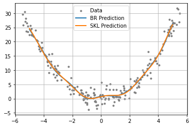
Plot the Results

We then plot the results for the two methods, and we should see that they produce nearly identical results.

import matplotlib
from matplotlib import pyplot as plt

fig = plt.figure()
ax = plt.axes()
plt.grid()

plt.scatter(X_train, y_train, marker=".", c="grey", label="Data")
plt.plot(X_test, np.real(y_pred1), linewidth=2, label="BR Prediction")
plt.plot(X_test, y_pred2, linewidth=2, label="SKL Prediction")

plt.legend()

plt.show()