Open an interactive version of this example on Binder:

Maximum Mean Discrepancy

This example demonstrates the maximum mean discrepancy using data drawn from two different distributions. Additionally, we demonstrate the empirical witness function, which displays the difference between the two distributions.

To run the example, use the following command:

python examples/kernel/maximum_mean_discrepancy.py

import numpy as np
from gym_socks.kernel.probability import maximum_mean_discrepancy
from gym_socks.kernel.probability import witness_function

from sklearn.metrics.pairwise import rbf_kernel
from functools import partial

Generate the Sample

Define the kernel function and generate the data.

We generate two samples, one from a Gaussian distribution and another from a Laplacian distribution to mimic the example from literature. Higher sample sizes will lead to a more accurate result.

sigma = 0.25
kernel_fn = partial(rbf_kernel, gamma=1 / (2 * (sigma ** 2)))

m = 5000  # sample size for P
n = 5000  # sample size for Q

X = np.random.standard_normal(size=(m, 1))
Y = np.random.laplace(size=(n, 1))

Compute the MMD

We then compute the maximum mean discrepancy using both the unbiased and biased statistics.

maximum_mean_discrepancy(X, Y, kernel_fn=kernel_fn, biased=True, squared=False)

0.06728449836826957

maximum_mean_discrepancy(X, Y, kernel_fn=kernel_fn, biased=False, squared=False)

0.06475312584455958

Plot the Witness Function

The witness function is used to view the difference between the two distributions.

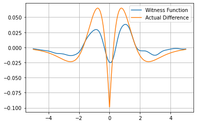
We plot the witness function, along with the true PDF of both the Gaussian and Laplacian distributions to illustrate the difference between the two samples. Intuitively, the witness function should have values closer to zero where the two distributions are similar, and have larger values (further from zero) where the distributions are dissimilar.

This depends on the kernel used, the kernel parameters (the bandwidth in the case of the RBF kernel), and the density of sample information (which is highest close to the mean, i.e. the witness function will be more accurate in areas where the sample density is high).

import matplotlib
import matplotlib.pyplot as plt

from scipy import stats

t = np.linspace(-5, 5, 1000).reshape(-1, 1)
z = witness_function(X, Y, t, kernel_fn=kernel_fn)

pdf_gaussian = stats.norm.pdf(t, 0, 1)
pdf_laplacian = stats.laplace.pdf(t, 0, 1)

fig = plt.figure()
ax = plt.axes()
plt.grid()

plt.plot(t, z, label="Witness Function")
plt.plot(t, pdf_gaussian, label="Gaussian PDF")
plt.plot(t, pdf_laplacian, label="Laplacian PDF")

plt.legend()
plt.show()

fig = plt.figure()
ax = plt.axes()
plt.grid()

plt.plot(t, z, label="Witness Function")
plt.plot(t, pdf_gaussian - pdf_laplacian, label="Actual Difference")

plt.legend()
plt.show()