Open an interactive version of this example on Binder:

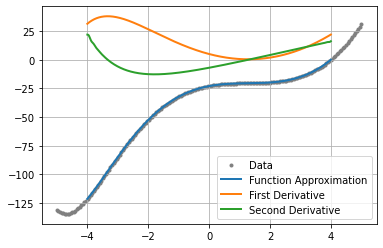
Derivative Approximation

This example demonstrates the use of conditional distribution embeddings to compute an approximation of the first and second derivatives of a function,

\[f(x) = x^{3} - 4 x^{2} + 6 x - 24 + \exp(-x)\]

We use an idealized dataset, which approximates the partial derivatives well. Introducing noise to the dataset creates fluctuations that needs to be offset by a higher regularization parameter and smoother kernel.

To run the example, use the following command:

python examples/kernel/derivative_approximation.py

import numpy as np
from functools import partial
from gym_socks.algorithms.kernel import ConditionalEmbedding
from gym_socks.kernel.metrics import rbf_kernel_derivative

from sklearn.metrics.pairwise import rbf_kernel
from sklearn.metrics.pairwise import euclidean_distances

from time import perf_counter

Generate the Sample

The following sample is idealized in order to demonstrate the technique. Additive noise causes fluctuations in the derivative approximation.

sample_size = 200
X_train = np.linspace(-5, 5, sample_size).reshape(-1, 1)
y_train = X_train ** 3 - 4 * X_train ** 2 + 6 * X_train - 24 + np.exp(-X_train)

# Uncomment the following line to incorporate noise in the sample.
# y_train += 10 * np.random.standard_normal(size=(sample_size, 1))  # Additive noise.

X_test = np.linspace(-4, 4, 1000).reshape(-1, 1)

Kernel and Parameters

sigma = 0.1
gamma = 1 / (2 * sigma ** 2)
kernel_fn = partial(rbf_kernel, gamma=gamma)
regularization_param = 1 / (sample_size ** 2)

Compute the Appromation

start = perf_counter()
alg = ConditionalEmbedding(regularization_param=regularization_param)
G = kernel_fn(X_train)
K = kernel_fn(X_train, X_test)
alg.fit(G)

C = rbf_kernel_derivative(X_train, sigma=sigma, distance_fn=euclidean_distances)
D = rbf_kernel_derivative(X_train, X_test, sigma=sigma, distance_fn=euclidean_distances)

y_pred = alg.predict(y_train, K)
y_pred_d1 = -alg.predict(y_train, K * D)
y_pred_d2 = alg.predict(y_train, (G * C) @ np.linalg.solve(alg._W, K * D))

print(perf_counter() - start)

0.10406230900025548

Plot the Results

We then plot the original function, the first derivative, and the second derivative against the original data.

import matplotlib
from matplotlib import pyplot as plt

fig = plt.figure()
ax = plt.axes()
plt.grid()

plt.scatter(X_train, y_train, marker=".", c="grey", label="Data")
plt.plot(X_test, y_pred, linewidth=2, label="Function Approximation")
plt.plot(X_test, y_pred_d1, linewidth=2, label="First Derivative")
plt.plot(X_test, y_pred_d2, linewidth=2, label="Second Derivative")

plt.legend()

plt.show()