Open an interactive version of this example on Binder:

Linear System ID

This example demonstrates the linear system identification algorithm.

By default, it uses the CWH4D system dynamics. Try setting the regularization parameter lower for higher accuracy. Note that this can introduce numerical instability if set too low.

To run the example, use the following command:

python examples/identification/linear_id.py

import gym_socks

import numpy as np

from gym.envs.registration import make

from gym_socks.algorithms.identification.kernel_linear_id import kernel_linear_id

from gym_socks.policies import ConstantPolicy
from gym_socks.sampling import sample
from gym_socks.sampling import sample_generator
from gym_socks.sampling import random_sampler

Configuration variables.

system_id = "CWH4DEnv-v0"
regularization_param = 1e-9
time_horizon = 1000

Generate the Sample

We generate a sample from the system, with random initial conditions and random actions. Increasing the sample size and reducing the regularization parameter will increase the accuracy of the approximation.

env = make(system_id)

sample_size = 100

state_sampler = random_sampler(sample_space=env.state_space)
action_sampler = random_sampler(sample_space=env.action_space)


@sample_generator
def sampler():
    state = next(state_sampler)
    action = next(action_sampler)

    env.state = state
    next_state, *_ = env.step(action=action)

    yield (state, action, next_state)


S = sample(sampler=sampler, sample_size=sample_size)

Algorithm

We then compute the system approximation using the sample.

alg = kernel_linear_id(S=S, regularization_param=regularization_param)

Using the known dynamics, we can validate the output of the algorithm against a known result. We simulate the system forward in time over a very long time horizon in order to observe how close the approximation is to the actual system dynamics.

For simulation, we choose to apply a constant policy, that applies the same control action at each time step.

policy = ConstantPolicy(action_space=env.action_space, constant=[0.01, 0.01])

env.reset()

# Set a specific initial condition for simulation.
initial_condition = [-0.75, -0.75, 0, 0]

# Simulate the system using the actual dynamics.
env.state = initial_condition
actual_trajectory = [env.state]
for t in range(time_horizon):
    action = np.array(policy(time=t, state=[env.state]), dtype=np.float32)
    obs, *_ = env.step(time=t, action=action)
    next_state = env.state

    actual_trajectory.append(list(next_state))

# Simulate the system using the approximated dynamics.
estimated_trajectory = [initial_condition]
for t in range(time_horizon):
    action = policy(time=t, state=[env.state])
    state = alg.predict(T=estimated_trajectory[t], U=action)

    estimated_trajectory.append(state)

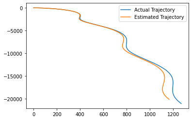
Results

We then plot the simulated trajectories of the actual system alongside the predicted state trajectory using the approximated dynamics.

import matplotlib
import matplotlib.pyplot as plt

fig = plt.figure()
ax = plt.axes()

actual_trajectory = np.array(actual_trajectory, dtype=np.float32)
plt.plot(actual_trajectory[:, 0], actual_trajectory[:, 1], label="Actual Trajectory")

estimated_trajectory = np.array(estimated_trajectory, dtype=np.float32)
plt.plot(
    estimated_trajectory[:, 0], estimated_trajectory[:, 1], label="Estimated Trajectory"
)

plt.legend()

plt.show()